Objective: We want to monitor the prediction of a recommender system usinf the UpTrain framework. Specifically, we want to check how close the predictions of the model are to the ground truth and also check if the model recommendations suffer from any biases (such as the popularity bias).
Dataset and ML model: In this example, we train a recommender system to recommend items to users based on their previous shopping history. The dataset is a subset of the and the model to train embeddings is the .
Note: Requires to be installed. We ran the following code successfully with Gensim version 4.3.0.
Step 1: Train the model
Each product has a unique stock-keeping unit (sku) that is used as a product identifier. We use to learn a embeddings corresponding to each sku based on shopping sessions of the user.
x_train_sku = [[e['product_sku'] for e in s] for s in data['x_train']]
model = Word2Vec(sentences=x_train_sku, vector_size=48, epochs=15).wv
Step 2: Define a custom monitor (cosine distance between embeddings of predicted and selected items)
Next, we define a custom metric where we want to monitor the cosine distance between embedding vectors of predicted and selected items. Specifically, we want to measure the cosine distance between the ground truth and first predicted item.
def cosine_dist_init(self):
self.cos_distances = []
self.model = model
def cosine_distance_check(self, inputs, outputs, gts=None, extra_args={}):
for output, gt in zip(outputs, gts):
if (not output) or (not gt):
continue
y_preds = output[0]
y_gt = gt[0]
try:
vector_test = self.model.get_vector(y_gt['product_sku'])
except:
vector_test = []
vector_pred = self.model.get_vector(y_preds)
if len(vector_pred)>0 and len(vector_test)>0:
cos_dist = cosine(vector_pred, vector_test)
self.cos_distances.append(cos_dist)
self.log_handler.add_histogram('cosine_distance', self.cos_distances, self.dashboard_name)
Step 3: Define another custom monitor (price difference between predicted and selected items)
Next, we also add a custom metric to measure the absolute log ratio between the ground truth and prediction item prices
def price_homogeneity_init(self):
self.price_diff = []
self.product_data = data['catalog']
self.price_sel_fn=lambda x: float(x['price_bucket']) if x['price_bucket'] else None
def price_homogeneity_check(self, inputs, outputs, gts=None, extra_args={}):
for output, gt in zip(outputs, gts):
if (not output) or (not gt):
continue
y_preds = output[0]
y_gt = gt[0]
prod_test = self.product_data[y_gt['product_sku']]
prod_pred = self.product_data[y_preds]
if self.price_sel_fn(prod_test) and self.price_sel_fn(prod_pred):
test_item_price = self.price_sel_fn(prod_test)
pred_item_price = self.price_sel_fn(prod_pred)
abs_log_price_diff = np.abs(np.log10(pred_item_price/test_item_price))
self.price_diff.append(abs_log_price_diff)
self.log_handler.add_histogram('price_homogeneity', self.price_diff, self.dashboard_name)
Step 4: Define the prediction pipeline
x_test = data['x_test']
y_test = data['y_test']
inference_batch_size = 10
def model_predict(model, x_test_batch):
"""
Implement the model prediction function.
:model: Word2Vec model learned from user shopping sessions
:x_test_batch: list of lists, each list being the content of a cart
:return: the predictions returned by the model are the top-K
items suggested to complete the cart.
"""
predictions = []
for _x in x_test_batch:
key_item = _x[0]['product_sku']
nn_products = model.most_similar(key_item, topn=10) if key_item in model else None
if nn_products:
predictions.append([_[0] for _ in nn_products])
else:
predictions.append([])
return predictions
Step 5: Define UpTrain config and initialize the framework
Step 6: Ship your model in production with UpTrain
for i in range(int(len(x_test)/inference_batch_size)):
# Define input in the format understood by the UpTrain framework
inputs = {'data': {"feats": x_test[i*inference_batch_size:(i+1)*inference_batch_size]}}
# Do model prediction
preds = model_predict(model, inputs['data']['feats'])
# Log input and output to framework
ids = framework.log(inputs=inputs, outputs=preds)
framework.log(identifiers=ids, gts=y_test[i*inference_batch_size:(i+1)*inference_batch_size])
# Adding 1 sec pause to visualize the results live on the dashboard
time.sleep(1)
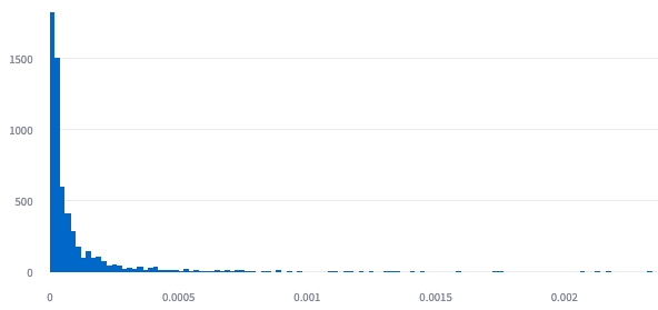
Histogram plot for items with popularity
From the UpTrain dashboard, we can find the histogram for popularity bias. We can see that most of the items that are recommended have low popularity. Our model does not look to be suffering from popularity bias.
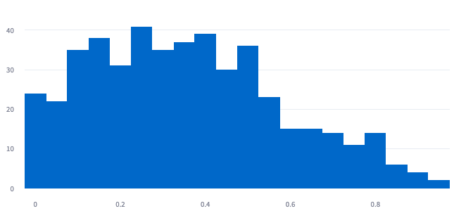
Histogram plot for cosine distance between ground truth and prediction
In the dashboard, we can measure the cosine distance between the embeddings of the recommended items and the items that were actually bought. A lot of them have zero cosine distance (implying that the recommendations were spot on). Also, we observe that the predictions are concentrated around the low cosine distance (< 0.4) space.
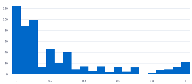
Histogram plot for absolute log price ratio between prediction and selected items
Finally, we also added a custom monitor where we wanted to check whether our model is providing outrageous recommendations (e.g., recommending washing machines when the user wants to buy just a washing detergent). In the below plot, we observe that the price range of most of the recommended items is close to the price of the actually bought item.